Tutorial
In this tutorial, you will learn how to use project “Sailor” to build your own algorithms and models from data stored in your SAP backends. In particular, you will learn how to:
Configuration
Before using the functions provided as part of project “Sailor,” you will have to configure the package to work with your SAP systems. For a detailed description of the configuration, please refer to the Getting started guide.
To start using project “Sailor,” execute the following commands to load the required packages. Since the standard data format that is used in project “Sailor” are pandas dataframes, we also import the pandas library. You can import the required packages like this:
import pandas as pd
from sailor.assetcentral import find_models, find_equipment, find_notifications, find_systems
Reading Master Data
To start the analysis, we first identify the equipment of interest. We use find_equipment() to search for the pieces of equipment
of interest - namely those belonging to the model my_model_name. The function returns a EquipmentSet,
an object representing multiple pieces of equipment. The convenience function as_df() returns a representation of the
EquipmentSet as pandas dataframe.
equipment_set = find_equipment(model_name='my_model_name')
equipment_set.as_df().head()
- Filtering data
Other ways of filtering are also available, e.g., for selecting the
my_model_nameequipment in a specific location, say PaloAlto:equipment_set2 = find_equipment(model_name='my_model_name', location_name='PaloAlto')
For an overview of the syntax used for filtering, refer to the documentation of the Filter Language. To get an overview of the fields that are available as filters, you can use the function
get_available_properties(). The fields in the resulting set can be used as filters. Similar functions also exist for the other objects:from sailor.assetcentral.equipment import Equipment Equipment.get_available_properties()
Furthermore it is possible to filter on result sets directly. Please see
filter()for details:equipment_set2.filter(id='ID_123')
Other typical starting points for the analysis are models. You can search for models using
find_models().
models = find_models(name = 'my_model_name')
You can then navigate to the equipment using find_equipment().
equi_for_model = models[0].find_equipment()
In case of equipment that is operated together and influences each other, the set of equipment is often modeled as System.
You can also start the analysis and exploration from a (set of) system(s) using find_systems().
systems = find_systems(name = 'my_system')
You can analyse events that have occured on the equipment, namely notifications that were created or workorders that were performed.
Let’s select all notifications that have been reported since August 2020. The find_notifications() function can be used to search
for notifications that are linked to the equipment in the EquipmentSet. The function returns a
NotificationSet,
which represents a set of notifications, similar to the EquipmentSet for equipment.
Again, a pandas dataframe representation of the object can be obtained using the as_df() function.
notification_set = equipment_set.find_notifications(extended_filters=['malfunction_start_date > "2020-08-01"'])
notification_set.as_df().head()
Exploring Data
To facilitate exploration and use of the extracted data for exploration, visualization, and model building, the as_df() function
is provided for all objects. The functions provide representations of the objects as pandas dataframe.
notification_set.as_df()
equipment_set.as_df()
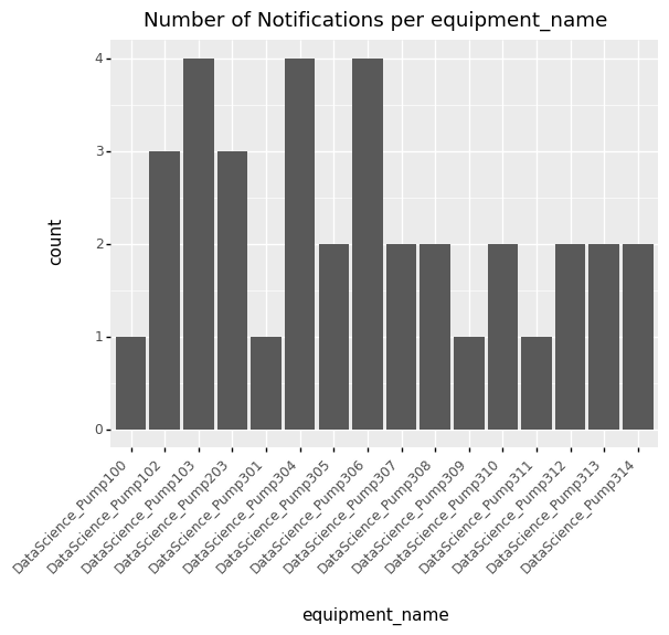
Convenience functions for typical plots are provided as part of the package. One of them is plot_distribution() for sets.
This function can be used to plot the value distribution of a set with respect to a specific parameter. For example, let’s
plot the distribution of notifications across equipment.
notification_set.plot_distribution('equipment_name')
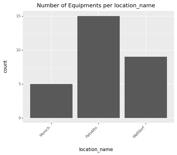
Along the same lines, we can plot the distribution of equipment by location.
equipment_set.plot_distribution('location_name')
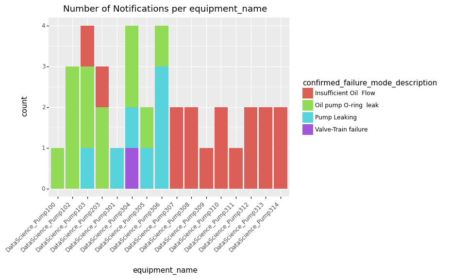
An additional parameter can be used to determine the coloring of the bars. All fields that are returned in as_df() can be
used in the grouping or coloring.
notification_set.plot_distribution(by='equipment_name', fill='confirmed_failure_mode_description')
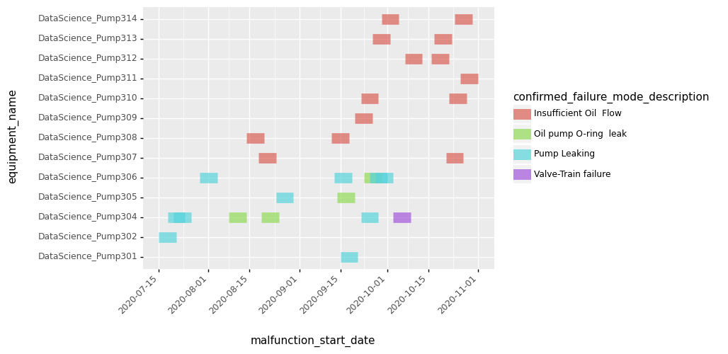
To visualize the distribution of notifications across equipment and time, the function plot_overview() may be used.
This will plot one row per piece of equipment associated with one of the notifications, the x-axis represents time. A colored block represents the time when
a notification was active on a piece of equipment, with the color representing the associated failure mode.
notification_set.plot_overview()
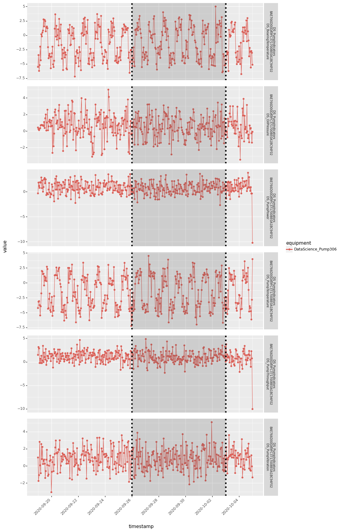
To understand whether there is an obvious pattern in the sensor data that is associated with a specific notification, the function
plot_context() can be used. This shows the behavior of all indicators associated with the equipment before, during, and after the
notification. This can be useful to understand whether there are obvious differences in the sensor data prior to the notifications
versus afterwards. This could help understand the issue associated with the notification.
notification_set[0].plot_context()
Note that this filters the data for the notification locally. So if you want to plot the timeseries data for multiple notifications, it might be more efficient to create a timeseries dataset locally as described in Read timeseries data and then pass it as parameter to plot context.
data = equipment_set.get_indicator_data('2020-05-01 00:00:00+00:00', '2021-03-01 00:00:00+00:00')
notification_set[0].plot_context(data)
Read Timeseries Data
For many use cases like anomaly detection, failure prediction, or remaining-useful-life prediction, it is useful to look at the machine’s sensor data. Sensor data is attached to equipment via indicators. An indicator is a description of measured values.
To find out which indicators are defined for a piece of equipment, you can use find_equipment_indicators()
indicators = equipment_set[0].find_equipment_indicators(name = 'my_indicator')
For a set of equipment, you can identify the set of indicators they have in common using find_common_indicators().
This might be useful if you want to do an analysis across multiple pieces of equipment.
indicators = equipment_set.find_common_indicators()
To retrieve timeseries data from SAP IoT for the indicators of interest, you use the function get_indicator_data().
This retrieves data for a single piece of equipment.
data = equipment_set[0].get_indicator_data('2020-05-01 00:00:00+00:00', '2021-03-01 00:00:00+00:00', indicators)
If you leave indicator set blank, then all indicators attached to the piece of equipment will be fetched.
For retrieving timeseries data for multiple pieces of equipment, it is more efficient to use the function get_indicator_data().
If here the indicator set is left blank, then all indicators returned by find_common_indicators() are queried.
data = equipment_set.get_indicator_data('2020-10-01 00:00:00+00:00', '2021-01-01 00:00:00+00:00')
Equally, it is possible to retrieve pre-aggregated data from SAP IoT. The function signature is very similar to the one above, but you can specify aggregation interval and aggregation functions.
interval = pd.Timedelta(hours=1)
data = equipment_set.get_indicator_aggregates('2020-10-01 00:00:00+00:00', '2021-01-01 00:00:00+00:00',
                                              aggregation_functions=['MIN', 'MAX'], aggregation_interval=interval)
Working with Timeseries Data
Timeseries data is always returned as a TimeseriesDataset.
With this object you have some options on how to work with the data contained within it.
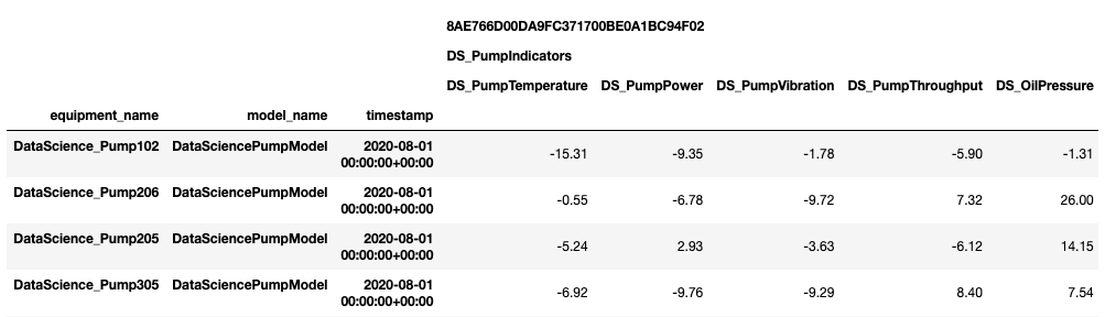
You can retrieve the data as a DataFrame:
data.as_df(speaking_names=True)
Filtering. E.g., filter the dataset based on a subset of indicators or equipments:
eq_subset = data.equipment_set.filter(location_name='PaloAlto')
ind_subset = data.indicator_set.filter(name=['DS_BearingTemperature', 'DS_OilPressure'])
data = data.filter(equipment_set=eq_subset, indicator_set=ind_subset)
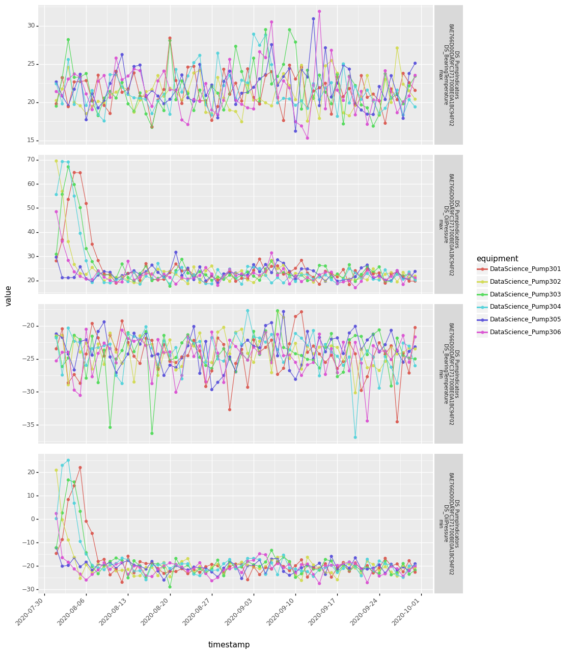
Aggregation and interpolation. If you are working with raw data and want to have your timeseries data aggregated.
Interpolation of NaN values is also supported:
data = data.aggregate('24h', ['min', 'max']).interpolate('24h')
Finally, you might be interested in plotting the resulting dataset:
data.plot()
Working with Systems
Systems are hierarchical data structures in AssetCentral. With SAP Predictive Asset Insights it is possible to create quite deeply nested system trees consisting of many systems and equipment. Retrieving these systems and the timeseries data associated with it can be a cumbersome task. Sailor provides some functionality to support data scientists in exploring systems.
Find systems and get indicator data:
ss16 = find_systems(name = ['JK0_SY0-1','JK0_SY0-6'])
data16 = ss16.get_indicator_data('2021-05-01','2021-05-07')
data16.as_df(speaking_names=True)
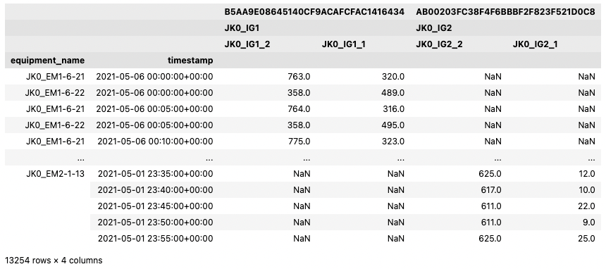
By default, the TimeseriesDataset contains every piece of equipment from every system encountered by traversing the trees of each system in the SystemSet.
Some indicators might not be used with some equipment. In these cases the values are set to NaN.
Analysis tables for systems
New in version 1.9.0.
Above representation answers the question: “which data is in my system?” In some cases a wide table format is preferred. E.g., for the training of machine learning models, it is desirable to to have all the indicator values of all the equipment grouped by system.
A wide analysis table can be created as follows:
from sailor.assetcentral.system import create_analysis_table
wide16 = create_analysis_table(ss16, data16)
wide16.as_df(speaking_names=True)
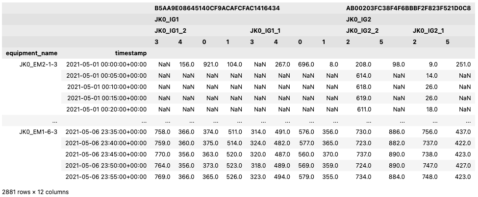
In a wide analysis table, all the information for a system and a timestamp is represented in a single row. Since one indicator can be assigned to multiple pieces of equipment, a uniquely numbered column is used to distinguish between the indicator instances that are created by such assignments. This number is unique within a single analysis table.
Each system is represented by a so called leading equipment as the equipment_name. Find the leading equipment for each system
by calling get_leading_equipment() on the SystemSet.
Writing Master Data
We also aim to provide the possibility to write data to all backend systems supported by Sailor. In this example we show you how to create notifications in AssetCentral.
Notifications are usually created for some equipment.
Therefore we can use the create_notification() function
to create a new notification for an equipment. In this example we want to create a new breakdown notification
with high priority:
equi = equipment_set[0]
notif = equi.create_notification(
                status='NEW', notification_type='M2', priority=25,
                short_description='Valve broken',
                start_date='2021-07-07', end_date='2021-07-08')
We might want to update this notification at a later time, e.g., when the maintenance crew is working on the equipment.
For this we need a notification object representing this notification. This can be the original notif object that
we have created, or you can obtain the object from Assetcentral again.
We can call the update() method directly on the
Notification object to send our desired changes to Assetcentral:
notif = find_notifications(id='previous_notification_ID')[0]
notif.update(status='IPR')
As you can see from these examples we can use the same properties as keyword arguments, that we are familiar with,
e.g., from when using the find_* functions.
Customization
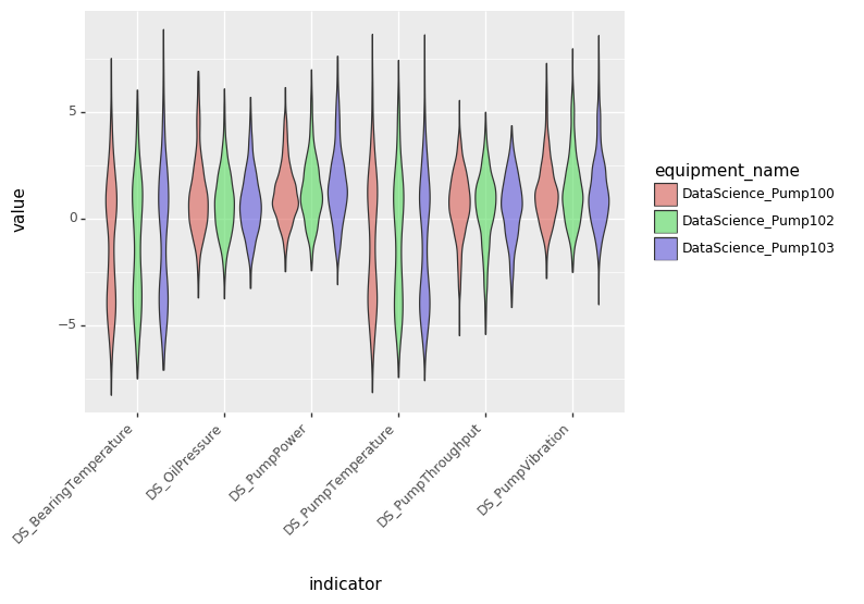
Building Custom Visualizations
To build your custom analysis or plot, you can use the data in any ResultSet and transform
it into a pandas dataframe using as_df(). The data frame can then form the
basis of your visualization.
import plotnine as p9
from sailor.utils.plot_helper import _default_plot_theme
data = equipment_set[0:4].get_indicator_data('2020-09-01 00:00:00+00:00', '2020-10-05 00:00:00+00:00')
df = data.as_df(speaking_names=True).droplevel([0, 1], axis=1).reset_index()
df = df.melt(id_vars=['equipment_name', 'model_name', 'timestamp'], var_name='indicator')
p9.ggplot(df, p9.aes(x='indicator', y='value', fill='equipment_name')) + p9.geom_violin(alpha=0.6) + _default_plot_theme()
Building Custom Machine Learning Models
Building machine learning models can be done using the same starting point as building custom visualizations, namely the method
as_df().
This is an example of the steps necessary to train an isolation forest for detecting anomalies in the timeseries data.
from sklearn.ensemble import IsolationForest
# find equipments and load data
equi_set = find_equipment(model_name='my_model_name')
data = equi_set.get_indicator_data('2020-09-01', '2020-10-05')
# train isolation forest
iforest = IsolationForest()
iforest.fit(data.as_df())
# score isolation forest, and join back to index (equipment/timestamp info)
score_data = data.as_df()
scores = pd.Series(iforest.predict(score_data), index=score_data.index, name='score').to_frame()